Profiler Stereo

Detailed: LSP Profiler Stereo (P1S)

Formats: CLAP, JACK, LV2, VST2, VST3

Categories: Utility

Developer: Stefano Tronci

Description: 

A simple plugin for audio systems profiling. The profiling is performed by an algorithm based on the Synchronized Swept Sine method by Antonin Novak.

The profiler plugin allows to profile audio systems. These properties of an audio system can be currently profiled:

• Latency.
• Linear Impulse Response.
• Nonlinear Characteristics.

A brief description of the plugin usage is provided below. For a summary of controls, see the Controls section.

1: Connection

The audio system to be profiled should be connected as in the measurement chain below:

• profiler output -> audio system input - audio system output -> profiler input

It is advisable to set the audio stack for stable operation (least amount of buffer over/underruns) when profiling. By default, in order to remove unwanted latency from the profile, the plugin operates a profiling sequence that includes latency detection. This will remove the average group delay of the entire chain above.

This might affect the accuracy of the phase response measurement of the audio system under test. If this is undesired, it is recommended to assess the systemless latency first, and disable automatic latency measurement during profiling. To do so, set up this latency measurement loopback:

• profiler output -> straight connection -> profiler input

More details are provided in Section 3.

2: Calibration

The plugin has a built-in calibration tone (sine wave) generator whose controls are accessible in the 'Calibrator' section. After the measurement chain in Section 1 has been realised, it is suggested to set all hardware level controls (if any) to -Inf dB and then enable the calibrator by pressing Enable in the 'Calibrator' section (led shines). This forces the plugin to transition into the CALIBRATING state, and the corresponding LED in the 'Results' section will shine.

Raise the hardware level controls and/or operate the calibrator Amplitude control until the Input Level meter provides a good level. All test signals levels will be set by the calibrator Amplitude control.

The test signals level is good when:

• The monitored plugin input is significantly higher than background noise.
• The calibration tone is not producing any unwanted distortion in the audio system.
• The calibration tone is not producing clipping in the plugin.

When the calibration tone is streaming, it is recommended to try a few different values of Frequency and select for the calibration the frequency that yields the maximum output of the audio system under test. The use of the frequency analyser plugin can facilitate this task.

After the calibration is concluded, the calibrator should be disabled.

3: Latency Measurement

The plugin automatically detects latency at each profiling cycle by default. However, there are cases in which it is advisable to measure latency only once, and disable Latency Detection from all subsequent profilngs. This is useful when:

• The phase response of the system under test needs to be profiled as accurately as possible.
• The signal level at which latency detection is most reliable is different from the level at which profiling is wanted.

To operate a one time latency measurement, set up the latency measurement loopback of Section 1. Then, measure latency once by pressing Measure in the 'Latency Detector' section, where all of the plugin Latency Detector controls are available. After a successful measurement, disable the latency detection from the system profiling sequence by pressing the Enable button (ensure the LED is off). By doing so the Latency Detection step will be omitted in subsequent profiling measurements, and the systemless latency will used to time align the result, thus preventing alteration of the system under test phase response.

One time latency measurements are also useful when the signal level for optimal latency detection is higher than that for system profiling. If this is the case, set the test signal amplitude for optimal latency measurement by operating the Amplitude control in the 'Calibrator' section, measure latency, disable the Latency Detector by disabling the Enable button in the 'Latency Detector' section, and reset the amplitude control to the optimal value for audio system response profile (as discussed in Section 2).

To be noted that, if the audio stack is not stable, buffer over/underruns (for example, JACK xruns) can produce change of latency and invalidate the one time latency measurement (for this reason latency is part of the profiling sequence by default).

Whenever the plugin is detecting latency, its state will be DETECTING LATENCY and the corresponding led in the 'Results' section will shine.

4: Set profiling test signal duration

The control Coarse Duration in the 'Test Signal' section is to be used to set the profiling chirp coarse duration. The actual chirp duration will be optimised during the pre-processing phase and shown in the Actual Duration indicator. Most measurements will be accurate with 10s Coarse Duration. Longer test duration increases the signal to noise ratio. If a reverberant system is being measured, the Coarse Duration should be longer than the expected reverberation time.

5: Perform the profiling

Pressing Profile in the 'Test Signal' section triggers a single profiling sequence. This will make the plugin to transition through the following states automatically:

• DETECTING LATENCY - In this state the latency of the audio system measurement chain is assessed. This step can be omitted by disabling the Enable toggle in the 'Latency Detector' section. If latency was never measured, the plugin will force latency detection.
• PREPROCESSING - In this state the plugin optimises the test signal parameters and generates the test chirp.
• WAITING - In this state the plugin waits for a time set by the Coarse Duration control. For reverberant systems, this time should be longer than the expected reverberation time. This waiting state avoids the reverberant tail of the Latency Detection chirp to pollute the measurement.
• RECORDING - In this state the profiling chirp is emitted and the audio system output recorded. A tail is also recorded in order to not truncate the high frequency reverberation recording.
• CONVOLVING in this state the plugin is convolving the recorded output with an inverse filter in order to calculate the characteristics of the audio system.
• POSTPROCESSING - In this state the measurement result is being analysed to extract properties.

The current state of the plugin is displayed at any time in the 'Results' section.

6: Post processing the results

Post processing is performed automatically after each measurement or manually by pressing the Post-process button in the 'Results' section. Whenever the plugin is postprocessing, its state will be POSTPROCESSING and the corresponding LED in the 'Results' section will shine. The post-processing steps can calculate:

• Background noise magnitude.
• Reverberation Time (RT).
• Energy Decay Linear Correlation coefficient.
• Coarse Linear Impulse Response Duration

All the quantities above are mostly relevant for linear time invariant (LTI) systems. The result will be displayed and postprocessed from the time originle of the Linear Impulse Response estimate of the system.

To change this, operate the Offset control in the 'Results' section, which allows to introduce a time offset. For numerical reasons, few details of the measured Linear Impulse Response are mapped into negative time samples to the left ot the origin of time. In case the spread of the Linear Impulse Response to the left of the origin of time is important, introducing a negative offset will increase accuracy of the calculations listed above, as well as providing a more accurate measurement. The Reverberation Time can be calculated with any of the algorithms in the RT Algorithm selector in the 'Results' section. All the algorithms are based in calculating, from the Linear Impulse Response, the Energy Decay curve through backward integration, fitting a straight line in the Energy Decay curve in a specified interval and solving for the point at which the straight line intercepts -60 dB from the peak energy.

See the RT Algorithm description for a list of the implemented algorithms, all based on ISO 3382-2 (but without filtering).

The algorithms supply the best results only if the background noise floor level in the Energy Decay curve is at least 10 dB below the lower limit of the regression line calculation. If this is true, the relevant Noise Floor LED will shine. In order to improve the Signal To Noise ratio, it can be advised to:

• Make sure there is not unwanted clipping or distortion, as distortion products inflate the background noise assessment.
• Make sure the profiling chirp duration is long enough, as longer chirps provide better Signal To Noise ratio.
• Make sure the amplitude is high enough with respect the background noise, but not so high to produce unwanted distortion.
• Make sure that eventual Linear Impulse Response samples to the left of the origin of time are not being omitted by introducing some negative offset.

The Energy Decay Linear Correlation coefficient is the Pearson correlation coefficient for the fitted regression line used for Reverberation Time calculation. For well fitted decaying lines this value is close to -1.

The Coarse IR Duration is instead the Linear Impulse Response duration based on the envelope of the Energy Decay curve. The value of the Coarse IR Duration is the time at which the envelope dives into the noise floor.

7: Saving the results

The profile can be saved by using the Save button in the 'Results' section. See Save Mode for the available saving modes. All saving ranges are rounded to the next tenth of second. Auto should be able to save all the meaningful parts of the Linear Impulse Response.

Whenever the plugin is saving to file, its state will be SAVING and the corresponding LED in the 'Results' section will shine.

Controls:

• Bypass - bypass switch, when turned on (LED indicator is shining), the plugin bypasses signal.

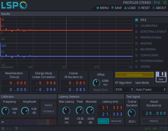
'Results' section:

• Results Graph - Graph that shows the Linear Impulse response, from the Offset value up to the Reverberation Time.
• PROFILER STATE - Shows the internal state of the plugin.
• Reverberation Time (s) - Indicator that reports the estimated overall Reverberation Time in seconds, according to the selected RT algorithm and Offset.
• Energy Decay Linear Correlation - Indicator that reports the Pearson correlation coefficient of the Energy Decay linear regression line used for Reverberation Time calculation.
• Coarse IR Duration (s) - Indicator that reports the coarse value of the Linear Impulse Response duration, estimated by Energy Decay envelope, in seconds.
• RT Algorithm - Reverberation Time (RT) is calculated by linear regression of the Energy Decay curve. The limits are chosen by this selector.
• EDT0 - Early Decay Time, Linear Regression algorithm on values of Energy Decay between 0 dB and -10 dB from peak.
• EDT1 - Early Decay Time, Linear Regression algorithm on values of Energy Decay between -1 dB and -10 dB from peak.
• RT10 - Reverberation Time, Linear Regression algorithm on values of Energy Decay between -5 dB and -15 dB from peak.
• RT20 - Reverberation Time, Linear Regression algorithm on values of Energy Decay between -5 dB and -25 dB from peak.
• RT30 - Reverberation Time, Linear Regression algorithm on values of Energy Decay between -5 dB and -35 dB from peak.
• Save Mode
• LTI Auto (*.wav) - Save, as a WAV file, the Linear Impulse Response from the Offset value up to the largest value of time between RT and Coarse IR Duration.
• LTI RT (*.wav) - Save, as a WAV file, the Linear Impulse Response from the Offset value up to to the RT value.
• LTI Coarse (*.wav) - Save, as a WAV file, the Linear Impulse Response from the Offset value up to the Coarse IR Duration value.
• LTI All (*.wav) - Save, as a WAV file, all the measured samples of Linear Impulse Response to the right of the Offset value.
• All Info (*.lspc) - Save, as an LSPC file, all the measured information.
• Offset - Introduce an offset from the origin of time of the Linear Impulse Response, for post processing purposes, milliseconds.
• Post-process - Button that forces the plugin to post-process the measurement result.
• Save - Save button.
• Noise Floor - If shining, the background noise and/or Offset value are optimal for the selected RT algorithm accuracy.

'Calibrator' section:

• Frequency - Frequency of the Calibration tone.
• Amplitude - Amplitude of the Calibration tone.
• Input Level (dB) - Indicator that reports the input level in dB.
• Enable - enables the Calibration tone.
• Feedback - If off, the feedback loop between input and output is disabled to avoid gain buildup.

'Latency Detector' section:

• Max latency - Maximum value of the expected transmission line latency, in milliseconds (needs to include buffering latency).
• Peak - Peak threshold for early detection: if the gap between consecutive local convolution peaks is higher than this value the plugin returns the latency associated with the highest peak.
• Absolute - Absolute threshold for the detection algorithm: values of convolution smaller than this are ignored by the algorithm.
• Latency (ms) - Indicator that reports the measured latency in milliseconds.
• Enable - Enables latency detection, if this control is deactivated, Latency Detection is omitted by the profiling sequence.
• Measure - Button that forces the plugin to perform a single latency measurement.

'Test Signal' section:

• Coarse Duration - Sets the coarse duration of the profiling Test Signal.
• Actual Duration - Actual duration of the profiling Test Signal, after optimisation performed in pre-processing.
• Profile - Button that forces the plugin to perform a single profiling measurement.